Compare Map Projections

[info]    Viewing options: South up    Flat oceans    Apply

The Wagner Bros.

Wagner’s Own Equal-Area Variations

In 1941, Karlheinz Wagner wrote a paper ^[1] showing the flexibility of the method of Umbeziffern and demonstrated it by presenting four different equal-area projection variants derived from the equatorial azimuthal projection.

The first of these four variants is nowadays well-known as Wagner VII (or Hammer-Wagner), but as far as I know, the other three have been mostly ignored. At least, I could not find a single reference to them in cartographic literature. Granted, this might well be due to the fact that I haven’t read that much cartographic literature. (And if you know of a source that is mentioning them: Please tell me!)
However, I’d like to show the variants here.

Don’t expect anything spectacular!
In the text, Wagner states his opinion that there’s little creative leeway for a useful world map. Consequently, he uses only slight modifications of the parameters.

For the lack of established names (see above), I’m going to call the variants Wagner VII.b to Wagner VII.d. The first variant, of course, is the well-known Wagner VII, which might be called VII.a in certain contexts to avoid confusion. But mostly, it’ll be better to just dismiss the suffixed lowercase letter for this variant.

The Böhm Notation that is shown at each projection is explained in the article about Umbeziffern.
The Geocart Paramaters are the values you’ll have to insert in the application Geocart (starting with v3.2) to render the corresponding variant. (The release date of that version hasn’t been announced yet.)
Wagner’s Spezifikation lists the values that Wagner added the the illustration’s caption in the article mentioned above.

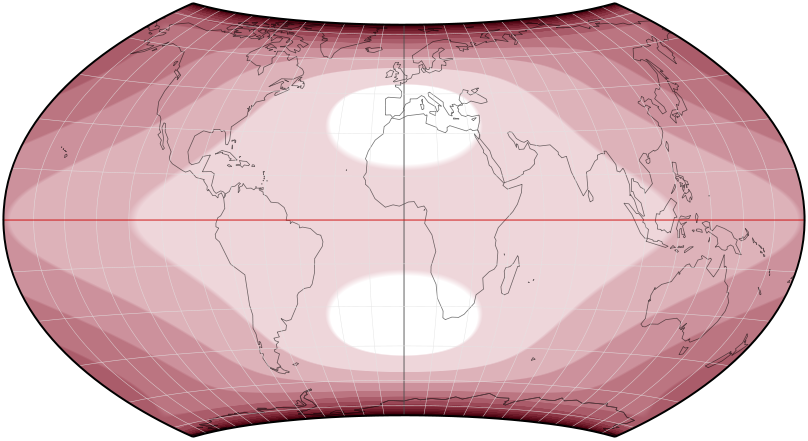
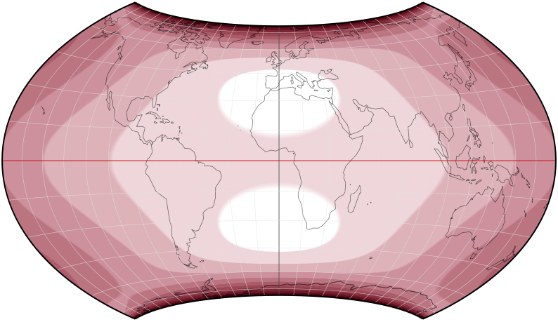
Moreover, I’ll add distortion visualization images (see short notes) which hopefully are interesting – but keep in mind that Wagner clearly stated:

Das beste Kriterium bei verhältnismäßig so geringen Unterschieden ist immer noch das Empfinden des geschulten Auges und nicht die mathematischen Verzerrungswerte.

The best criterion when dealing with such comparatively small differences still is the perception of the trained eye rather than mathematical distortion values.

 

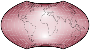
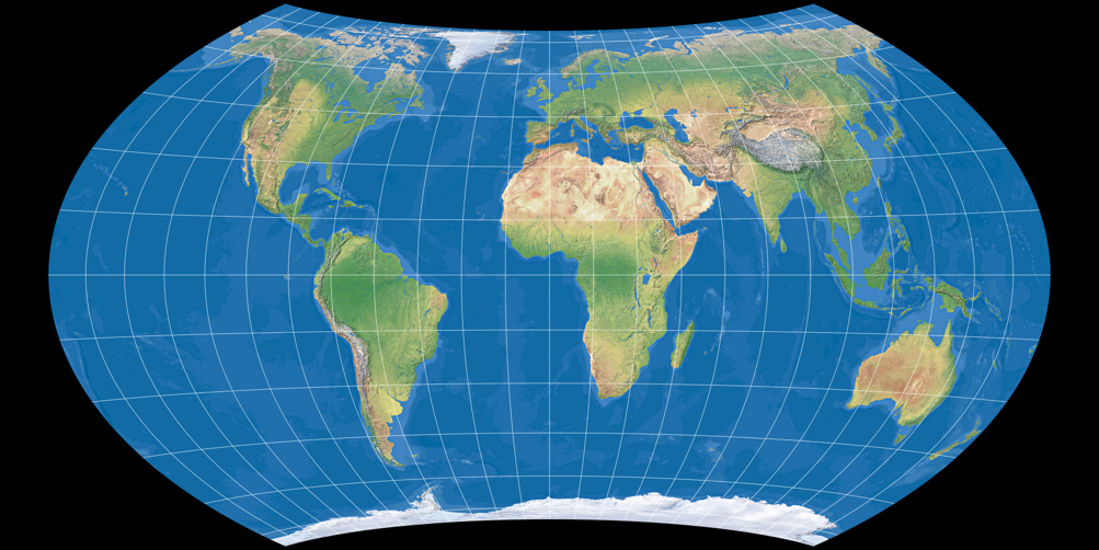
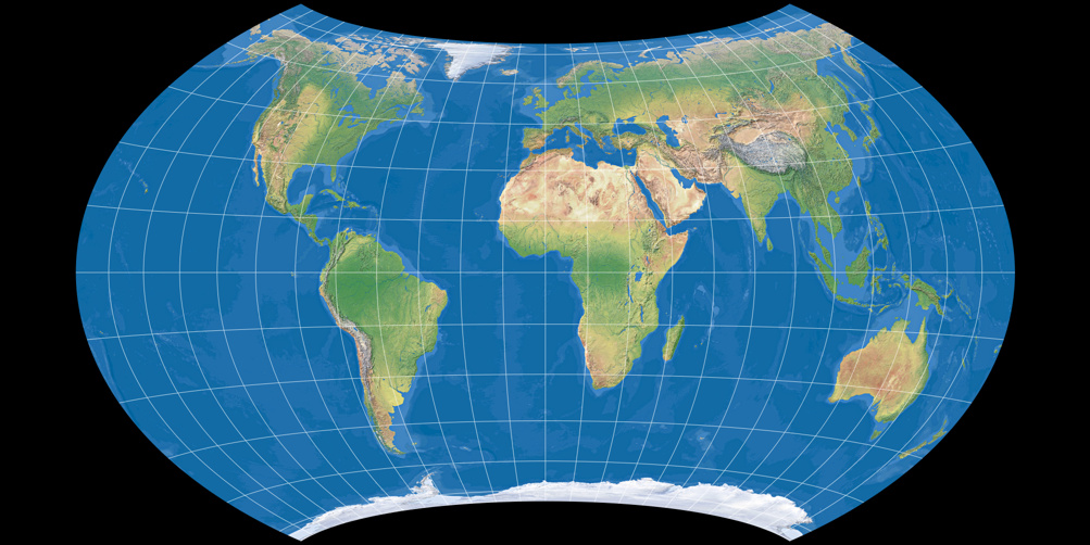
Wagner VII

The well-known Wagner VII.
Presumably, this was Wagner’s personal favorite variant, regarding that he lists it first and that in his 1949 text book Kartographische Netzentwürfe he didn’t show the other three. Nonetheless he pointed out that all four of them will be appropriate in the field of cartography.

Wagner VII	Open with WVG-7
Böhm Notation:	65-60-60-0-200
Geocart Parameter:	a = 2.667233, b = 1.241036, m = 0.906308, m2 = 1, n = 0.333333
Wagner’s Spezifikation	prime meridian/equator = 1/2 n = λ₁/180 = 60/180 = 0.33333… m = sin φ₁ = sin 65° = 0.90631… k = 1.46602…    (see note below)

 

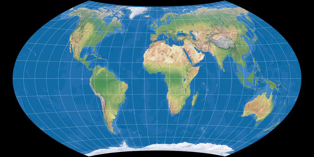
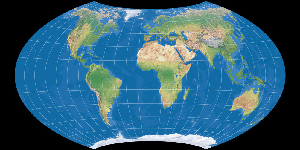
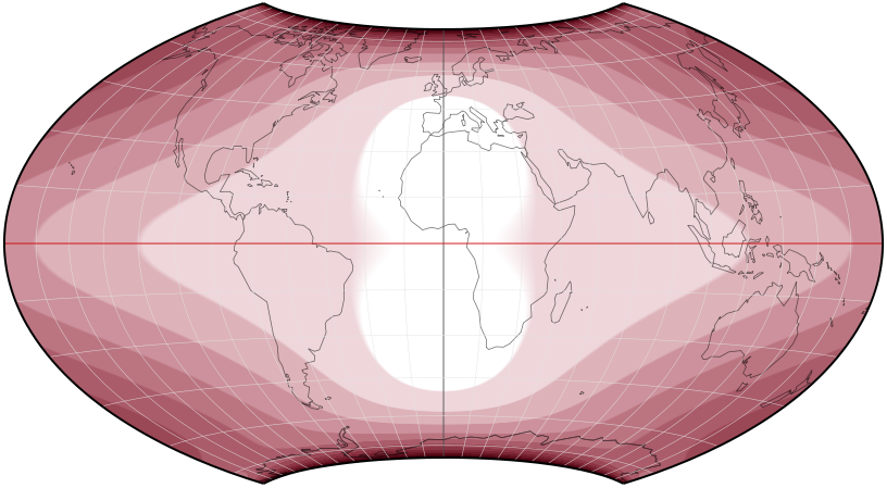
Wagner VII.b

The variant VII.b carefully increases the pole line length and the bending of the meridians. Apart from that, the central meridian is compressed slightly – Wagner will keep this modification on the two following variants.
You have to look closely to spot the differences to VII.a.

Wagner VII.b	Open with WVG-7
Böhm Notation:	61-65-60-0-205.128
Geocart Parameter:	a = 2.476901, b = 1.278296, m = 0.87462, m2 = 1, n = 0.361111
Wagner’s Spezifikation	prime meridian/equator = 0.975/2 n = λ₁/180 = 65/180 = 0.36111… m = sin φ₁ = sin 61° = 0.87462… k = 1.374449…    (see note below)

 

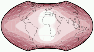
Wagner VII.c

In this case the pole line gets shorter while the bending of the meridians gets furtherly increased. Wagner commented that personally, he preferred the first two variants because of the lesser bending, but I have to say that VII.c is my favorite among these four configurations! I like that it improves Africa’s shape and that Greenland seems a little less »squished«.

Wagner VII.c	Open with WVG-7
Böhm Notation:	67.5-75-60-0-205.128
Geocart Parameter:	a = 2.205242, b = 1.177984, m = 0.92388, m2 = 1, n = 0.416667
Wagner’s Spezifikation	prime meridian/equator = 0.975/2 n = λ₁/180 = 75/180 = 0.41667… m = sin φ₁ = sin 67° 30′ = 0.92388… k = 1.36751…    (see note below)

 

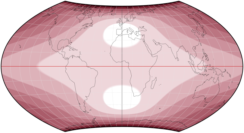
Wagner VII.d

The pole line length is increased again to get nearly as long as in the VII.b, while the curvature of the meridians is even more pronounced than in the c variant.
Note the distortion characteristic in the four corners of the map, e.g. at Alaska! This indicates a direction that we’ll meet again in the pending fifth (and hopefully, final) part of the Wagner article series.

Wagner VII.d	Open with WVG-7
Böhm Notation:	60-80-60-0-205.128
Geocart Parameter:	a = 2.036056, b = 1.276034, m = 0.866025, m2 = 1, n = 0.444444
Wagner’s Spezifikation	prime meridian/equator = 0.975/2 n = λ₁/180 = 80/180 = 0.44444… m = sin φ₁ = sin 60° = 0.86602… k = 1.24733…    (see note below)

 

Comparison Matrix

Since the differences between the variants are minor indeed, here’s a table which lets you directly compare each variant to each of the others:

	Wagner VII	Wagner VII.b	Wagner VII.c	Wagner VII.d
Wagner VII	—	VII vs. VII.b	VII vs. VII.c	VII vs. VII.d
Wagner VII.b	VII.b vs. VII	—	VII.b vs. VII.c	VII.b vs. VII.d
Wagner VII.c	VII.c vs. VII	VII.c vs. VII.b	—	VII.c vs. VII.d
Wagner VII.d	VII.d vs. VII	VII.d vs. VII.b	VII.d vs. VII.c	—

 

See you soon!

In the fifth part of this article series I’ll talk about the Wagner variants by Canters, Böhm and Aribert Peters. Since they’re already shown on this website (see thumbnail list), I can make it short. And then this Wagner series will be finished at last!
Unless of course something additional comes to my mind…    ;-)

 
 

A Note regarding the k-Values

If you open the variants in the WVG-7 and compare the k-values from Wagner’s specification mentioned above to the k₁-values of Canters’s notation over there, you’ll notice: They are equal on the Wagner VII but differ slightly on the other three variants. In theory, they should always be identical!
I’ve got three possible explanations for this phenomenon:

1. I can’t rule out the possibility that I did something wrong then I calculated the values, however I’m fairly certain that this is not the case.
2. There are errors in Wagner’s paper. I know that sounds unlikely, but there are definitively some printing errors in the text, so why not here? And meanwhile I’m quite convinced that for VII.b and VII.c, Wagner calculated the k-Value for an axial ratio of 1/2, then changed his mind and used a ratio of 0,975/2 and simply forgot to adjust the k-value in his manuscript.
3. On Wagner VII.c, the difference between Wagner’s value and the one I calculated is small enough to assume it’s just a matter of rounding errors.

 

References

1. ↑ Wagner, Karlheinz:
   Neue ökumenische Netzentwürfe für die kartographische Praxis.
   In: E. Lehmann, ed., Jahrbuch der Kartographie 1941.
   Leipzig: Bibliographisches Institut. 176–202.

Back to Selected Projections  •  The Wagner Projections (Part 3)  •  Go to top